Category: astrostatistics

Research on inference, nested sampling, MCMC, machine learning

  • Information Field Theory

    Prompt to Claude Sonnet 4.6: “Critically examine NIFTY and the “information field theory” framework of Enßlin. Is it essentially Gaussian processes as parent distributions of relatively simple hierarchical Bayesian models, and the major difference to standard methods is MGVI/geoVI being a higher order VI method, or are there important other contributions other than rebranding.”

    What IFT/NIFTY Actually Claims to Be

    Enßlin’s Information Field Theory positions itself as “statistical field theory applied to signal reconstruction,” drawing an analogy between Bayesian inference on fields and quantum/statistical field theory. The marketing language is substantial, so it’s worth decomposing what is genuinely novel versus what is repackaging.


    The Core Statistical Structure

    What the framework reduces to

    You are largely correct in your characterization. The essential statistical structure is:

    Prior: A Gaussian process (or hierarchical model with GP at the base) P(s)=G(s,S) where S is the signal covariance (the “power spectrum” in IFT language).

    Likelihood: Typically Gaussian or Poisson, often with a linear forward model P(d∣s)=G(d−Rs,N)

    Posterior inference: Approximation of P(s∣d)

    The “field theory” language (propagators, Feynman diagrams, action functionals) maps directly onto standard GP regression / Bayesian linear inverse problems:

    IFT terminologyStandard statistics
    Signal field sLatent function / GP draw
    Power spectrum Pk​Covariance kernel in frequency domain
    Response RForward/observation operator
    Information Hamiltonian H(s)=−logP(s,d)Negative log joint = energy
    Wiener filterPosterior mean under Gaussian prior + Gaussian likelihood
    Propagator DPosterior covariance

    The Wiener filter solution m=D⋅j, D=(S−1+R†N−1R)−1 is classical (Wiener 1949, and well-known in geostatistics as kriging). The “free theory” of IFT is literally Gaussian process regression.

    Verdict on the base framework: The re-expression in field-theoretic language is pedagogically interesting for physicists but does not add statistical content. It is Gaussian processes (and their hierarchical extensions) written in physics notation.


    Where Things Get More Substantive

    1. MGVI and geoVI — the genuine methodological contribution

    This is where the framework has made arguably its most concrete methodological contribution that goes beyond rebranding.

    Standard VI approximates P(s∣d)≈q(s∣λ) by minimizing KL divergence, typically with a mean-field Gaussian q, which:

    • Ignores posterior correlations
    • Severely underestimates uncertainty in high dimensions

    MGVI (Metric Gaussian Variational Inference) [Knollmüller & Enßlin 2019]:

    • Approximates the posterior Fisher metric (natural gradient) to define a local Gaussian approximation
    • The key idea: use the prior as the variational metric, expanding around a latent mean
    • This gives an implicit full-covariance Gaussian in the standardized coordinates without explicitly storing the covariance matrix
    • The computational trick: work in the “white” space where the prior is N(0,I) via reparameterization, so the Jacobian of the natural gradient is tractable

    geoVI [Frank et al. 2021] extends this by:

    • Fitting a non-Gaussian approximation via a geometric transport — finding a map from a standard Gaussian to the posterior
    • The approximating family is richer than a Gaussian: it’s defined by a nonlinear transport map sampled via an ODE
    • This is closer to normalizing flows / transport-based VI but with specific structure exploited

    Is this genuinely higher-order? Yes, in a specific sense:

    • MGVI is essentially a natural gradient VI method with an implicit full-covariance structure exploited via the reparameterization trick — this avoids O(N2) covariance storage
    • geoVI captures non-Gaussian posterior geometry beyond second-order approximations
    • The connection to the Fisher metric / information geometry is used constructively, not just decoratively

    Comparison to other high-dimensional VI:

    • Similar in spirit to ADVI (Kucukelbir et al.) but with better-motivated geometry
    • Related to Laplace approximation but iterated and with uncertainty propagation
    • Related to EP (Expectation Propagation) but formulated variationally
    • The “implicit” full covariance via reparameterization has parallels in doubly reparameterized gradients and linear response methods

    The genuine contribution here is making full-covariance Gaussian VI tractable in high-dimensional function spaces where storing Σ is impossible, by exploiting the structure of the prior.

    2. The Operator/Linearization Framework in NIFTY

    NIFTY (Numerical Information Field Theory) implements inference over function spaces in a way that is relatively carefully structured:

    • Resolution independence: Fields are discretized but inference targets the continuum limit; the framework tracks how quantities scale with grid resolution
    • Operator algebra: Linear operators (R, S, etc.) are composed without explicitly forming matrices — this matters practically in high dimensions
    • Automatic differentiation through forward models: Not unique to NIFTY but well-integrated

    This is similar to what Gaussian process libraries (GPflow, GPyTorch) do, but with more explicit attention to the function-space limit and physical forward models. The comparison is closer to Firedrake/FEniCS + GP inference than to standard sklearn-style GP regression.

    3. Correlated Field Model

    The hierarchical prior on the power spectrum — where the spectral density itself has a prior (lognormal process over k-space) — is a recurring NIFTY pattern. This is:

    • A hierarchical GP model (GP prior on the log-power-spectrum)
    • Practically important for real data where the covariance structure is unknown
    • Similar to spectral mixture kernels (Wilson & Adams) or non-parametric Bayesian spectral estimation

    Not a major conceptual breakthrough, but a practically useful default prior structure with principled motivation.

    4. Feynman Diagram / Perturbative Expansion

    IFT uses the formal apparatus of QFT perturbation theory to compute non-Gaussian corrections to the Wiener filter. The “interacting field theory” corresponds to non-Gaussian priors or likelihoods expanded around the Gaussian “free theory.”

    Assessment: This is a genuine technique — using Feynman diagrams for approximate Bayesian inference via cumulant expansions exists in the statistics literature (e.g., Opper & Winther’s work on TAP equations, Plefka expansion in spin glasses). The IFT framing makes this natural for physicists but:

    • The same expansions are reinvented from the statistics/ML side multiple times
    • For serious non-Gaussianity, the perturbative expansion is of limited practical use (diverges or requires many terms)
    • In practice, the NIFTY applications mostly use MGVI/geoVI rather than perturbative corrections

    Critical Assessment

    Legitimate contributions

    1. MGVI/geoVI: Genuinely useful, reasonably novel VI methodology for high-dimensional field inference — competitive with or better than alternatives for structured inverse problems
    2. Resolution-independence / operator formulation: Useful engineering for large-scale inference problems, though similar ideas exist in the GP/PDE community
    3. Unified language for a class of problems (radio astronomy, CMB, medical imaging) that reduces coding overhead for domain scientists

    Legitimate criticism

    1. Terminological inflation: Renaming the posterior covariance “propagator” and the negative log-posterior “Hamiltonian” adds cognitive load for statisticians without adding content. The analogy to QFT is suggestive but imperfect — fields in IFT are finite-dimensional after discretization; Feynman diagrams here are glorified Taylor expansions of a log-posterior.
    2. Overclaiming novelty relative to GP literature: The core models are GP regression and hierarchical GPs. The power-spectrum inference is related to decades of work in geostatistics (variogram estimation), time series (Bayesian spectral analysis), and machine learning (kernel learning). Citations to this literature are sometimes sparse in IFT papers.
    3. The “field theory” framing doesn’t do much work in practice: Actual NIFTY applications use MGVI/geoVI (standard VI machinery), not perturbative Feynman diagrams. The perturbative IFT machinery is rarely deployed in real analyses.
    4. Comparison to mature alternatives is sometimes missing: For many problems IFT/NIFTY addresses, Laplace + HMC, EP, or properly implemented ADVI would be competitive. Careful ablations against these are not always present.
    5. Community somewhat siloed: The framework has been developed largely within a specific astrophysics group; cross-fertilization with the GP/probabilistic ML literature has been limited in both directions.

    Where it is genuinely valuable

    For the target audience — astrophysicists doing large-scale imaging inverse problems (e.g., VLBI imaging with eht-imaging, CMB reconstruction) — NIFTY provides:

    • A concrete, working implementation
    • Sensible default priors for smooth fields
    • A VI engine that handles millions of parameters better than naive approaches
    • Domain-specific forward models

    This is real value, even if the conceptual framework is largely a repackaging of GPs + hierarchical Bayes + VI.


    Summary Verdict

    ClaimAssessment
    IFT is fundamentally new statisticsNo — it is GPs + hierarchical Bayes in physics notation
    The Feynman diagram formalism adds practical valueRarely — it’s a perturbative approximation rarely used in practice
    MGVI/geoVI are genuine contributionsLargely yes — tractable full-covariance VI in high-dimensional function spaces with good geometric motivation
    The operator/resolution-independence framework adds valueYes, modestly — useful engineering, not unique
    The field theory framing is usefulFor physicists: yes pedagogically; for statisticians: adds noise

    Your characterization is approximately correct: the major statistical innovation is in the variational inference methodology (MGVI/geoVI), not in the prior/model structure. The latter is essentially hierarchical Gaussian processes. The “information field theory” branding is partly repackaging, though the repackaging serves a real community need and the VI work stands on its own merit.
  • Replace “using AI” with “using interpolation”

    (2nd try after HN feedback)

    When cloud computing was a new, cool buzzword thrown around that no one understood, a shortcut was suggested whether it is the right solution:

    In any sentence, replace “in the cloud” with “on another person’s computer”.

    “Computing on the cloud” becomes “computing on another person’s computer”.
    “I backup my data to the cloud” becomes “backup to another person’s computer”.
    This makes it easier to weigh benefits – they provide more space, and provide maintenance, against drawbacks – they have your data and fully control the computer it sits on.

    Today, “AI” is thrown around as an all-encompassing buzzword. “Enhance your start-up with AI”, “AI helps prepare lawsuit”, “AI-written lawsuit contains mistakes”, “Fighting wildfires with the help of AI”, “Get data insights with AI”.

    A shortcut to clarify thinking about AI

    To expose overuse of the term “using AI” without meaning, I propose to replace it with “using interpolation”: “Enhance your start-up with interpolation”, “Using interpolation helps prepare lawsuit”, “Interpolated lawsuit contains mistakes”, “Fighting wildfires with the help of interpolation”, “Get data insights with interpolation”.

    This makes a few things clear: First, there are the benefits of any automatic data processing approach; this is not new with AI. Secondly, the replacement is effective at stripping away the mythical meaning of “AI” as an independent actor, removing the possibility to delegate ownership to it. Saying “my interpolation did it” sounds today much sillier than “my AI did it”.

    Many, but not all AI methods can indeed be framed as interpolation, with a very complicated, high-dimensional distance function among outputs, to determine what to produce given an input. This distance function, or slatent space, was shaped from data.

    The interpolation framing reveals the first question to ask:

    1. Where do the underlying data come from, who made them?

    This first question leads you to problematic biases in the training data that the AI inherits. It can also reveal copyright issues and whether the data producers are fairly compensated.

    Now you are also more plainly seeing someone saying “I’m doing X with technique Y, ” which leads to the question: Is this better than what was there before? This is actually a two-part question:

    2. By what performance metric do the claimants want to be judged?

    This second question reveals what people value, and whether this aligns with your values.

    3. Is the performance better in that metric than the current method?

    Question three reveals whether there was an improvement made so far, and may help distinguish vaporware from genuine improvement. The baseline may be another AI method, for example comparing LLMs to Markov Chains trivially reveals how much better LLMs are. Only very few analyses truly lack a baseline.

    Conclusion

    Demand from AI articles to know the data origin, performance metric, and historic baseline.

    If they don’t give that information, replace “using AI” with “using interpolation.”


    Postscript:

    Note that I did not include “what is the model?”, i.e., the architecture or training procedure – this is the least important technical detail.

    Questions 1) and 3) are often not made by the claimants, but reused. This is often not or extremely briefly described, reflecting how much time the AI developers spent on it. These three questions are essential for putting the AI claim into context.

    Some cop-outs:

    • If only similar performance is achieved, the AI developers often point to improvements in processing time, which should be added to the performance metric answer of question 2. It’s a valid goal to achieve somewhat comparable performance at much faster speed.
    • My pet peeve cop-out is “it has potential for improvement in the future.” This may be technically true, because models might learn with more training data. However, at least in a scientific and policy context a opportunity for critically and objectively examining the outcome, in context of the historical baseline, is being skipped.
  • Replace “using AI” with “using computers”

    When cloud computing was a new, cool buzzword thrown around that no one understood, a shortcut was suggested whether it is the right solution:

    In any sentence, replace “in the cloud” with “on another person’s computer”.

    “Computing on the cloud” becomes “computing on another person’s computer”.
    “I backup my data to the cloud” becomes “backup to another person’s computer”.
    This makes it easier to weigh benefits – they provide more space, and provide maintenance, against drawbacks – they have your data and fully control the computer it sits on.

    Today, “AI” is thrown around as an all-encompassing buzzword. “Enhance your start-up with AI”, “AI helps prepare lawsuit”, “AI-written lawsuit contains mistakes”, “Fighting wildfires with the help of AI”, “Get data insights with AI”.

    Is there a similar shortcut that clarifies thinking?

    To expose overuse of the term “using AI” without meaning, I propose to replace it with “using computers”: “Enhance your start-up with computers”, “Using computers helps prepare lawsuit”, “Computer-written lawsuit contains mistakes”, “Fighting wildfires with the help of computers”, “Get data insights with computers”.

    This makes a few things clear: First, there are benefits to using computers because of their automatic data processing. This is not new with AI. Secondly, the replacement is effective at stripping away the mythical meaning of “AI” as an independent actor, removing the possibility to delegate ownership to it. Saying “my computer did it” sounds today much sillier than “my AI did it”.

    So, replace “using AI” with “using computers”. It reveals to you how little the statement by itself tells you.

    To seriously talk about AI, we have to unpack the term. In general terms, we are talking about methods that expand their capabilities with increasing data. Therefore to judge whether AI is good or not for an application, we need to find out:

    1. Where do the data come from, who made them?
      • Question 1 leads you to problematic biases in the training data that the AI inherits. It can also reveal copyright issues and whether the data producers are fairly compensated.
    2. By what performance metric do the claimants want to be judged?
      • Question 2 reveals what people value, and whether this aligns with your values.
    3. Is the performance better in that metric than the current method?
      • Question 3 reveals whether there was an improvement made so far, and may help distinguish vaporware from genuine improvement. The baseline may be another AI method, for example comparing LLMs to Markov Chains trivially reveals how much better LLMs are. Only very few analyses truly lack a baseline.

    Note that I did not include “what is the model?” – this is the least important technical detail.

    Questions 1) and 3) are often not made by the claimants, but reused. This is often not or extremely briefly described, reflecting how much time the AI developers spent on it. These three questions are essential for putting the AI claim into context.

    Some cop-outs:

    • If only similar performance is achieved, the AI developers often point to improvements in processing time, which should be added to the performance metric answer of question 2. It’s a valid goal to achieve somewhat comparable performance at much faster speed.
    • My pet peeve cop-out is “it has potential for improvement in the future.” This may be technically true, because models might learn with more training data. However, at least in a scientific and policy context a opportunity for critically and objectively examining the outcome, in context of the historical baseline, is being skipped.

    Demand from AI news articles to know the data origin, performance metric, and historic baseline.

    If they don’t give that information, replace “using AI” with “using computers.”

  • Publication time in astronomy vs statistics

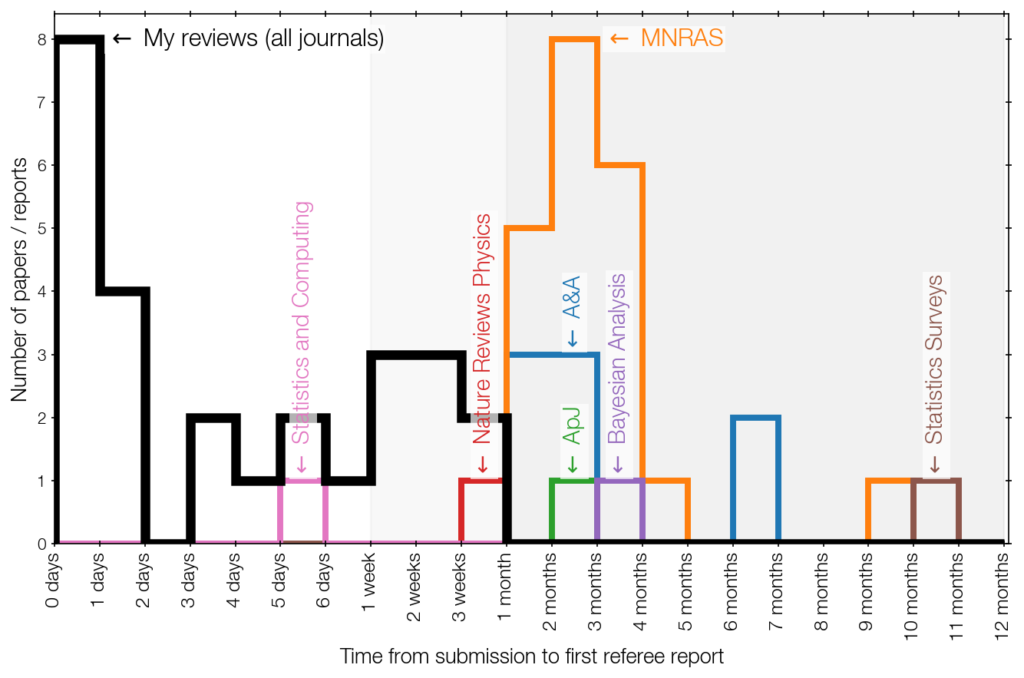
    After submitting a paper to an astronomy journal like MNRAS, ApJ, A&A, PASP it is quite typical to receive a referee report within 1-2 months.

    A search of my emails confirms this – green, orange, blue histograms are astronomy journals:

    For statistics journals, the waiting times can be much longer in my experience. For Statistics Surveys, and another paper not shown in the above, I waited for almost a year! That’s quite a shocking cultural difference. What do statisticians do all day?

    I also plotted in black how long I take between receiving a request for reviewing and submitting the review. I typically do it on the same day or the next.

    I am apparently not a typical reviewer!

    Oh – this might be a way to identify me as your reviewer 🙂

    (more…)
  • The top and bottom halves of data analysis in astrophysics

    There are two approaches to analysing data, which I will call the bottom and top half.

    Bottom half

    Look at images and data by eye. Discover anomalies and outliers. Argue primarily qualitatively. Potentially preprocess the anomaly-finding with machine learning.

    It’s a good approach for junior scientists to start looking at data (a) and understand its artifacts and limitations. However, the by-eye approach does not permit quantifying false positives and false negatives.

    The bottom half brought us the hunt for high-redshift galaxies and quasars, reddened quasars, the most luminous galaxy, the most massive black hole, Voorwerpjen, etc. etc.

    The bottom half is great for discovery of extremes by appearance.

    The bottom half approach can only search across data space, not by physical parameters. After discovery, to get physical information for the discovered system, one then switches to another type of analysis.

    Top half

    Use a physical model to fit data. Build a model that can explain the data. Quantify, including the uncertainties. Distinguish two competing physical processes.

    This can be achieved with (hierarchical) Bayesian models combined with advanced inference engines (nested sampling and dynamic Hamiltonian Monte Carlo), and more recently, perhaps, with simulation-based inference.

    Combining both halves

    Some research projects can use only the bottom half, discover something and argue qualitatively. It’s somewhat quite easy to do this: You just project the data into one or two dimensions – for example looking at color – and start visually inspecting the extremes. Slightly fancier versions, but conceptually the same, are to look at a latent space, for example produced by UMAP (or the older T-SNE), or an auto-encoder. These latent spaces are usually meaningless themselves, and randomly oriented so that a retraining gives something completely different. I’ve seen many researchers get lost in over-interpreting the shapes in latent spaces.

    To go beyond discovery and qualitative existence proofs, one needs the other half: An approach that models the demographics, placing the extremes in context, and connecting the physical space to the data space with a physically meaningful model.

    Admittedly, I call this bottom and top half to make myself and my focus on the top half feel superior. However, the top half can also not exist without the bottom half: You cannot do a blind, automated model fitting without investigating data artifacts, and careful validity checks. You need detailed analyses of individual, nearby galaxies to understand surveys of the distant Universe. So only the two halves make a whole.

  • How to get emotionally attached to software but leave no impact to science

    How do people get emotionally attached to software?

    I mean positively emotionally attached to the point of plastering stickers on their laptop, or negatively attached to the level of raising their voices in discussions.

    Here I explore a few causes that I have seen.

    1. Attachment to strict teachers

    This cause of attachment is common with compilers (Rust, Stan) and program provers. They nitpick and force you into a lane. After significant investment and boxing your problem into the right shape, they are given the green light like a priest giving you a blessing. You are now a member.

    The harsher the teacher, the more rigorous the trial, the more attached is the feeling of belonging to an elite club of survivors.

    2. Attachment to what you have spent building

    Just spending a lot of time building something causes you to be attached to it. Firstly, design decisions can be personal expressions. Secondly, after spending many long nights or even months working on it, there is a sunken cost. It’s hard to consider that you have “wasted” your time. If someone tells you, “why don’t you use tool Y”, you’d laugh it off, not even trying to learn tool Y because you understand your imperfect work of love.

    A more open minded point of view is to think of the “sunken cost” as an investment to deeply understand the challenges in that domain. Even if the developer drops the tool and switches over to something else, they now know the concepts and challenges deeply, at an expert level.

    Unconvincing value propositions

    Building new software is fun! Because of the two points above, the author is likely to proselytize around, trying to convert people to their great tool.

    The expressed value propositions can harbor a communication mismatch: The inside view of the developer is not the outsider view. Their values of “it is well understood” and “easy to change” do not translate to the next person who has not edited the software yet. Likely, the outsider has also seen a few people proselytize, and then the difference in value may be difficult to see.

    Work without impact to science

    Every week there are papers on arXiv where someone invested months of work on a new data analysis technique and finally finds that it does not outperform the classic benchmark.

    Sometimes this is stated outright. I think it is great science to try something new. But there are other cases.

    Sometimes the benchmark is a setting unlike how the analysis will be applied in the future (for example: complete data, spectroscopic redshifts, known noise), or the benchmark statistic is non-standard to the field. In any case, whether the new technique is better or worse, the abstract invariable ends with “And therefore, our technique is a promising platform for future data sets.”

    It is disheartening to think of the many person months wasted, because people did not think longer about what they should optimize for.

    Personal reflection

    I think I also suffer from some sunken cost w.r.t. nested sampling. It is quite addictive for me to think about algorithm variations.

    That “no one uses my software” is not a problem I have though. What keeps me grounded is seeing a clear need in conference and hallway dialogs, combined with critical thinking to crystallize out what the core question is.

  • The state of nested sampling research in 2026: II) Fundamental algorithm research

    see also part I.

    Nested sampling as an algorithm has a few papers presenting convergence proofs. It’s interesting from how many angles people have looked at this problem. See the relevant section in the literature review.

    Diagnostics (ongoing)

    Andrew Fowlie proposed an elegant test for diagnosing live whether nested sampling is sampling in an unbiased fashion, by tallying where in the likelihood-ordered list of live points the replacement point lands (I tend to confuse the wods order and rank). A variant is the statistically more powerful U-test ( section 4.5.2. of Buchner 2023). But ultimately, neither of these are as sensitive as you would wish.

    In practice, the most powerful technique is still observing the log(Z) value across reruns, e.g., when increasing the number of steps of the slice sampling procedure.

    More research is still needed on diagnostics. I suspect that the gradients of the dead points can be compared to the growth of the L-V curve and that could be more powerful.

    In the meantime, I transferred MCMC diagnostics to nested sampling, specifically the Jump Distance which traces the first-order autocorrelation length of a random walk. This research appears to be trivial for statistics journals and too non-astronomy for astronomy journals.

    Plauteaus (solved?)

    When the likelihood has plateaus, the original algorithm had an issue. In practice, this mostly occurs if your log-likelihood function returns a fixed number such as -1e300 when the parameters are invalid. Pragmatically, one can make that penalty slant towards the good region. More generally, an auxiliary with a tiny likelihood slant is a solution to plateaus, but in any case the nested sampling variant where all points with the same lowest likelihood value are removed has been proposed and should be the standard nested sampling method people implement (it is in UltraNest).

    Live point inheritance

    In most implementations, the dead point is replaced by sampling a new point, starting from another live point. This is true for ellipsoidal nested sampling and MCMC-based replacement schemes.

    In multi-modal settings, removing points can remove all points of a mode, and this was discussed early in the literature, mostly casually in conference proceedings (which I cannot find anymore, help!).

    Recently, I used analysis techniques from genetics to analyse the occurrence probability of mode die-out in nested sampling. The result is not analytic, but gives a simple rule of thumb, which I think is basically always fulfilled. So: do not worry about this!

    End-to-end proofs

    A limitation of current theoretical analyses is that most of these assume faithful likelihood-restricted prior sampling (LRPS). How can we go beyond this?

    Brendon Brewer solved this by embedding nested sampling within an MCMC framework. Fine, but most people do not use nested sampling that way.

    For nested sampling with step samplers, a key paper is “Unbiased and Consistent Nested Sampling via Sequential Monte Carlo” by Queensland University of Technology researchers Robert Salomone, Leah South et al., which present a proof by placing nested sampling within the sequential nested sampling umbrella of well-built-out theoretical analysis. There is a hole in that paper, which they are clear about: In SMC, there is a kernel which refreshes all points, while in NS, only one specific point is replaced. And so the connection is as of yet almost, but not quite, there.

    For nested sampling with region samplers, I just put out a theory paper analysing the replacement sampling space with Binomial point processes, which is the exact right tool for the job. This analysis is on the path to a end-to-end convergence proof of nested sampling, or at least bounding the errors.

    The nice aspect of convergence analyses is that once you have them, you know what you can tune. It does not work the other way around …

    By my recent count, there are over 6000 citations to the top 4 nested samplng packages. As machine learning becomes more prevalent, nested sampling analyses are used as the ground truth to compare against. Both of these facts should be justification to thoroughly understand nested sampling. Now we just need astronomers, statisticians and computer scientists to allocate funding for this research.

  • The state of nested sampling research in 2026: I) Scaling nested sampling to high-dimensions

    Since I wrote a systematic literature review (arxiv, scholar) in 2023, and written or contributed to several nested sampling packages, I’m someone who people turn to and ask, “what is next in nested sampling research”?

    In this first part, I will write about scaling nested sampling to high-dimensions.

    Contrary to conventional wisdom, nested sampling does not have poor scaling with dimensionality at all. If the prior equals the posterior, i.e., no information gain, the algorithm terminates successfully immediately, with high effective sample size.

    Two difficulties occur with the high information common with large datasets and hierarchical Bayesian models, where we learn an enormous amount of information. This can be easily seen with prior predictive checks – every prior realisation is plausible, but the observations are each highly peculiar in their own way, requiring a lot of fine tuning of the parameter space to find the posterior. This implies many nested sampling iterations, because in nested sampling, the number of iterations times the number of live points is proportional to the information gain: sqrt(N*K)=H

    The second difficulty is that the likelihood-restricted prior sampling used may scale poorly with dimensionality. The best technique so far is hit-and-run Monte Carlo (HARM) – miscalled slice sampling – first proposed used T Jasa & N Xiang – but introduced in detail by Will Handley’s PolyChord. Slice sampling is somewhat of a misnomer because we are not sampling the slice height, and in classical slice sampling one samples one dimension at a time. In any case, such MCMC approaches scale with dimensionality in a theoretically simple but practically difficult-to-understand way. One needs to tune M, the number of MCMC steps until the next point is decorrelated from the starting location (a random live point). Realistically the minimum M may be different throughout the run, but the worst-case will dominate and thus sets M which sets the compute budget. Annoying.

    Here are the current approaches:

    1. Make the run code faster – this is engineering: Some hacks here include vectorization, analytic marginalisation of variables not explicitly needed, and changing programming language. 2 research groups work on jax-based nested sampling implementations and parallelising. From an algorithm point of view, there is nothing here. Good marketing though …
    2. Focus on convex likelihoods: proximal nested sampling, ~1 researcher focused on imaging. This is an interesting approach not taken up by other research groups, yet.
    3. Give up on doing it right the first time and anneal towards the answer.
      • Diffusive nested sampling frames NS sampling as a MCMC process, with 1 active researcher (Brendon Brewer). The range of proposals within Diffusive Nested Sampling has not yet been fully explored, and a jax-based implementation would be good. I’ve had no luck getting the algorithm to behave though.
      • Snowballing nested sampling: Instead of expanding the number of steps until you get a nicely behaved run, expand the number of live points with a fixed number of steps.

    In my opinion, one of the most powerful techniques for making nested sampling run fast with many parameters is prior predictive checks. Often, the prior is misspecified, and information gain is unnecessarily high. Start from a reasonable prior.

    In high dimensions, you should also ask yourself whether the parameters have a meaning. If you are dealing with millions of pixel parameters and morphology, what are you doing? Do you really want to do Bayesian model comparison or do you just not know any other model comparison methods that may be a better fit?

    But what can you do. “High-dimensional inference” sounds cool and important, but I believe other inference axes are also worth pursuing, such as high information gain inference, phase transition inference, multi-modal inference.

    Because of the change in nature of the parameters, I don’t think nested sampling is the ideal algorithm for high-dimensional inference. My go-to-methods are

    a) divide and conquer importance resampling (as for example in PosteriorStacker). This is suitable for hierarchical models with low-dimensional per-object parameter spaces with medium to high information-gain per object. The parent distribution parameter space can be high dimensional.

    b) dynamic HMC. I’ve seen several people die on the hill of getting Stan to fit realistic astronomy models though. Differentiable programming with instrument responses is tough.

    The aversion of statisticians to nested sampling because they prefer SMC and the aversion of astrophysicists to SMC is a bit funny, given how close they are among the family of Monte Carlo algorithms. SMC requires some tuning of the tempering schedule, but has the advantage that one can potentially skip ahead to the posterior bulk. This is desirable for impatient researchers, such as those working on Gravitational Wave detections. A recent interesting paper was SMC+NUTS by Demasi+26.

    see also part II.

  • Simulation-based inference for X-ray astronomy

    In simulation-based inference, you train a neural network with pairs of model parameters θ and correspondingly data D, (θ, D). In the case of NRE, the network is a classifier, which predicts the probability that the data came from the (θ, D) stream corresponding to the joint p(θ,D) vs. a scrambled-up (θ, D) stream, corresponding to the respective priors p(θ)*p(D). With some algebra, this gives you p(D|θ), i.e., the likelihood. In the case of NPE, the network predicts p(θ|D) using a normalising flow, by optimizing the probability function to output most probability weight where θ is for the given D.

    The stream of (θ, D) is created by defining a prior p(θ), and a generator function D|θ which simulates data. Easy. Standard “forward-folding” (astronomer-speak) or generative modelling (statistician-speak).

    This scheme works well in a ML setting, where you have many tuples (θ, D), ideally, billions. Yes, you need a lot of data. This training cost hinders iterative model building.

    You can reuse standard industry network architectures to handle image data easily.

    Limitation 1: Varying observing conditions

    The scheme does not fit if you have variations in observing conditions. For example, if your instrument behaves slightly differently for each observation.

    Varying observing conditions are pervasive in X-ray astronomy because the object position on the focal plane changes the instrument response, both in the spectral and imaging sense. In optical astronomy, the equivalent is that you have different seeing conditions (filters are not considered time-variable). So we need to deal with this.

    [Aside on backgrounds: The background can also vary with position and time, which matters unless you are studying X-ray binaries and feel brave. The background can be simulated as well, with extending both θ and D, to background parameters and background region data, so this is not a deal-breaker.]

    The standard method then would be to either sample a random observing condition, and generate (θ, D), which would marginalise over the observing condition. Not wrong, but would lose information. The standard optical method is to derive the seeing conditions in the data analysis step from point sources in the image (e.g., SourceExtractor, photutils). This is reasonably fast. For X-ray astronomy, this is not possible, because the response is not location-invariant, so you cannot transplant information from nearby to the source.

    The proper way would be to sample not just p(θ, D), but p(θ, D | C) where C are the observing conditions, and define a conditional SBI (NRE or NPE) that gives its results conditional on an input C. If C was just the exposure time, and PSF FWHM, then we could make it part of D and sample it, and at inference time condition on it. However, in X-ray astronomy, C is a response matrix, and it is not trivial to smoothly sample from it, or to inform a SBI neural network about how to use it, because the SBI does not forward-fold. I suppose one could project C into a low-dimensional space.

    In any case, the samplings of C would likely be incomplete, and a new observation may not lie inside, erasing much of the cost savings at inference time that SBI should bring.

    Limitation 2: Poisson count data

    Why are there so few SBI – and, more generally – neural network papers with X-ray data? I think it is because neural networks suck with count data.

    You would think that you take a standard network that works with continuous data trained and knowing the L2 loss is proportional to a negative log-likelihood of a Gaussian switch for the loss for a negative log-likelihood of a Poisson and your done. But try to apply it to count data, and no, it doesn’t work. Why not? That’s a interesting ML research question. Correctly specified loss does not mean a trainable loss.

    So X-ray ML astronomers are hacking around by making X-ray count data Gaussian-like by smoothing, losing information in the process, or testing with trivial high-count situations.

    But once you bin finely enough in time or spectral channels (think XRISM, X-IFU), you are in the low count regime at least in those bins and have to deal with it.

    In my personal opinion, SBI is worth pursuing, but there are alternative approaches as well that scale to high dimensions that are not losing information. In any case, neural networks play a role, but it matters how you use them. Yes, I am being coy here on what is better, I’d like to be funded to resolve these issues.

  • Applied Computer Science and “Real” Physics

    In Computer Science, there is a divide between general methods research (such as: algorithms, data structures, security research) and applications (find a solution for a company or societal problem). When studying at University, I was surrounded by the opinion that the more general method is of higher value, and the other is “just application” and messy. I held this opinion for a while, too.

    In physics, there is a divide between software method research (such as: new data analysis methods) and finding out something about a physical process (application of a method to a specific case and interpreting the result). The latter is much higher regarded. I’ll give some examples I have experienced:

    1. Physicists would say “But what’s the new physics here?” and consistently display a dismissive attitude to automating, robustifying or generalising analyses.
    2. Astronomy journals reject papers that present general methods research without application.

    There is a cognitive dissonance there too, because methods papers are very highly cited. Physicists find them extremely useful. For example, the 2014 paper of PyMultiNest/BXA and the 2021 paper of UltraNest have 1500 and 500 citations, respectively.

    Pure data (catalog) papers are somewhere in the middle. They receive a substantial number of citations and moderate regard. But physicists would recommend not to publish a pure catalog paper with no direct scientific content.

    Part of the above can be explained by people liking similar people. If you are a computer scientist at a University, likely you are doing general research and hold that in high regard. If you are a physicist famous for some subfield, you will value progress in that subfield, not general-purpose methods that could help all fields.

    The tide is changing a bit recently. There are a few professorships for astrostatistics and machine learning in astronomy. And of course, the above is a simplification: there have been well-regarded experts in methods before, for example specific simulation techniques, observation techniques (direct imaging), going at least back to Joseph Fraunhofer developing the best optics.